Figures

Various figures, both interactive and non-interactive, related to the DiSCoVeR algorithm as applied to compounds and clusters. For more details, see the ChemRXiv paper.

Compound-wise and cluster-wise interactive figures produced via Plotly.

Hover your mouse over datapoints to see more information (e.g. composition, bulk modulus, cluster ID). Alternatively, you can download the html file at mat_discover/figures and open it in your browser of choice.

Compound-Wise

Pareto Front Training Contribution to Validation Log Density Proxy

Pareto Front k-Nearest Neighbor Average Proxy

Pareto Front Density Proxy (Train and Validation Points)

Cluster Properties

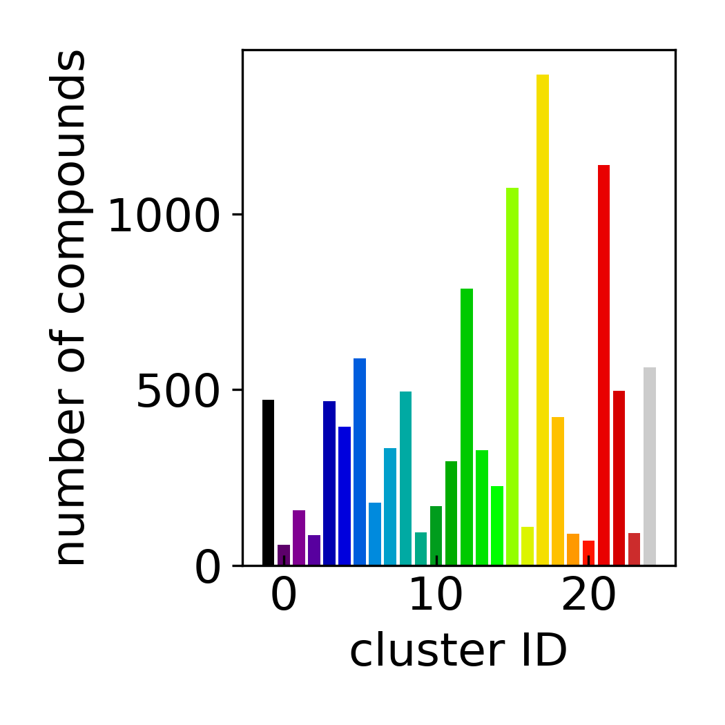
Cluster Count Histogram

DensMAP Embeddings Colored by Cluster

Cluster-Wise

Pareto Front Validation Fraction

Leave-one-cluster-out Cross-validation k-Nearest Neighbor Average Parity Plot

Density and Target Characteristics

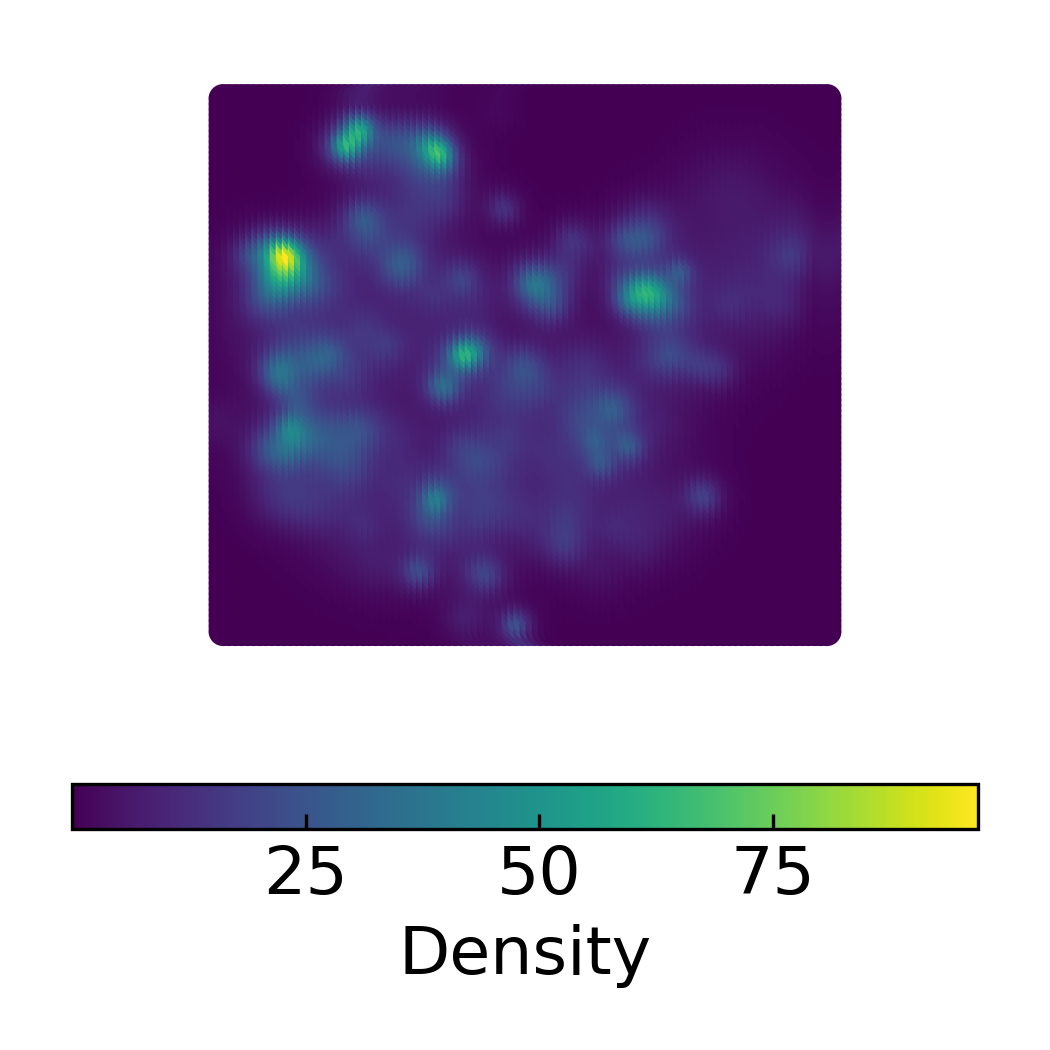
Density Scatter Plot of 2D DensMAP Embeddings

Target Scatter Plot of 2D DensMAP Embeddings

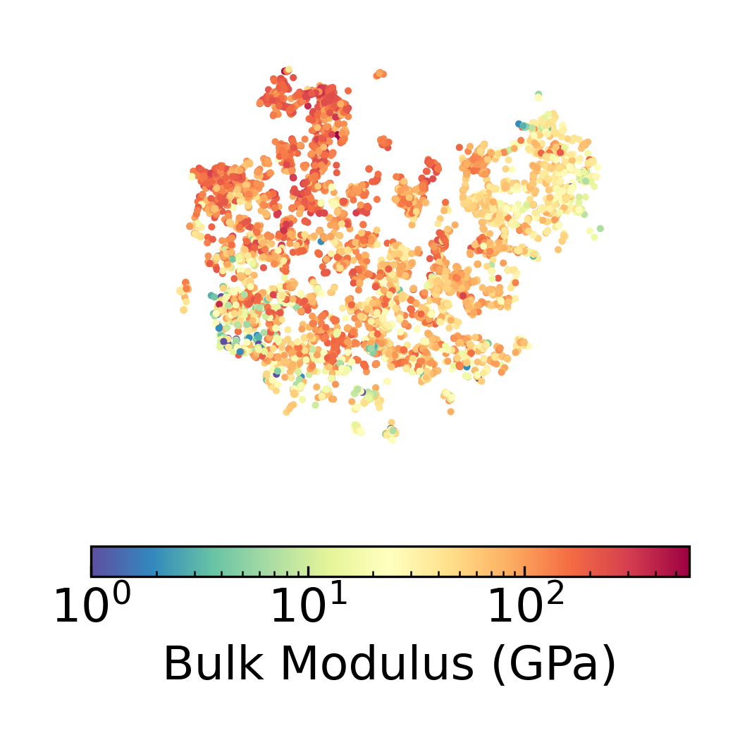
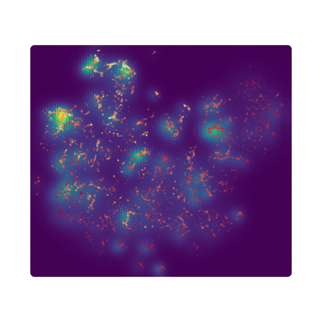
Density Scatter Plot with Bulk Modulus Overlay in 2D DensMAP Embedding Space

Adaptive Design Comparison

Take an initial training set of 100 chemical formulas and associated Materials Project bulk moduli followed by 900 adaptive design iterations (x-axis) using random search, novelty-only (performance weighted at 0), a 50/50 weighting split, and performance-only (novelty weighted at 0). These are the columns. The rows are the total number of observed “extraordinary” compounds (top 2%), the total number of additional unique atoms, and total number of additional unique chemical formulae templates. These are the rows. In other words:

• How many “extraordinary” compounds have been observed so far?

• How many unique atoms have been explored so far? (not counting atoms already in the starting 100 formulas)

• How many unique chemical templates (e.g. A2B3, ABC, ABC2) have been explored so far? (not counting templates already in the starting 100 formulas)

Random search is compared with DiSCoVeR performance/proxy weights. The 50/50 weighting split offers a good trade-off between performance and novelty.

In a similar vein using 300 adaptive design iterations, we compared the 50/50 DiSCoVeR algorithm with sklearn.neighbors.LocalOutlierFactor (novelty detection algorithm) using mat2vec and mod_petti compositional featurizers. LocalOutlierFactor (LOC) was only used for the novelty metric, i.e. the performance metric was computed as normal using CrabNet in both cases. Random search is also in there as a baseline. While LOC does reasonably well with finding new chemical formula templates and adding new atoms, it’s not very good at finding high-performing candidates (at least with this quick implementation of this). Perhaps this is because LOC isn’t suggesting candidates which improve the model’s predictive accuracy or because the LOC scores keep getting rescaled to certain range. Contrast this with Bayesian optimization which naturally favors exploitation over exploration as the optimization progresses, and DiSCoVeR which imitates this by using the same Scaler object instantiated during the first iteration. Technically, LOC uses the same Scaler instantiated in the first iteration, but that’s a moot point if LOC is already rescaling the values internally. In contrast, the 50/50 DiSCoVeR algorithm does well at optimizing both chemical novelty and performance.